First Steps: Acetone in Water
Introductory tutorial to perform QM/MM simulations using MiMiC on a small system, composed of an acetone molecule in water.
Main steps:
Calculate the dipole moment of acetone in vacuum
Solvate the system and equilibrate it with classical MD
Prepare the input for MiMiC and perform a QM/MM MD simulation at room temperature
Calculate the average dipole moment from selected snapshots of the production run
Estimate the difference between the dipole moment in vacuum and the one at room temperature to understand the effects of solvent and temperature
![]() This tutorial shows how to run a QM/MM MD simulation with MiMiC from scratch, including the equilibration of the system with classical MD. If you are already familiar with these preliminary steps, you can directly start from the Section QM/MM MD with MiMiC. All the files generated during these preliminary steps useful to start a QM/MM simulation are provided.
This tutorial shows how to run a QM/MM MD simulation with MiMiC from scratch, including the equilibration of the system with classical MD. If you are already familiar with these preliminary steps, you can directly start from the Section QM/MM MD with MiMiC. All the files generated during these preliminary steps useful to start a QM/MM simulation are provided.
![]() This tutorial assumes the user to have running versions of MiMiC, CPMD and GROMACS.
This tutorial assumes the user to have running versions of MiMiC, CPMD and GROMACS.
Instructions to install the MiMiC Framework (the MiMiC library and the MiMiC communication library) can be found in the Installation/MiMiC Framework section.
Instructions to install the CPMD and GROMACS with MiMiC enabled can be found in the Installation/External Programs section.
Instructions to install the MiMiCPy can be found in the Installation/MiMiCPy section.
![]() Tutorial based on:
Tutorial based on:
CPMD tutorial for the BioExcel Summer School on Biomolecular Simulations 2018 in Pula (Italy) from Bonvin Lab.
MiMiC tutorial from 2018 by Viacheslav Bolnykh
 and Emiliano Ippoliti
 Updates on the MiMiC tutorial (February 2021) and MiMiCPy documentation by Bharath Raghavan
CECAM Flagship School: Multiscale Molecular Dynamics with MiMiC (July 18-22, 2022 at CECAM HQ, EPFL, Lausanne, Switzerland)
![]() Main contributors to the updated version of this tutorial:
Main contributors to the updated version of this tutorial:
Andrea Levy
Sophia Johnson
Bharath Raghavan
Sonata Kvedaravičiūtė
David Carrasco de Busturia
System Preparation
Acetone is the organic compound with the formula (CH3)2CO, representing the simplest example of ketone. It is a colorless, volatile, flammable organic solvent naturally occurring in plants, trees, forest fires, vehicle exhaust, and as a breakdown product of animal fat metabolism. It dissolves in water and is used to make plastic, fibers, drugs, and other chemicals, and also to dissolve other substances.

![[Image source]](https://en.wikipedia.org/wiki/Acetone#/media/File:Acetone-3D-balls.png)
For this tutorial we will assume that you downloaded the corresponding git repository, hence you will have the provided folders and files in the same locations.
curl https://gitlab.com/mimic-project/mimic-docs/-/archive/main/mimic-docs-main.tar.gz?path=docs/tutorials/AcetoneTutorial -o AcetoneTutorial.tar.gz
tar --strip-components=3 -zxvf AcetoneTutorial.tar.gz
The above commands downloaded a copy of the exercise repository AcetoneTutorial in the current folder. Navigate the repository and create your own directory to run this exercise
cd AcetoneTutorial
mkdir solution
cd solution
Dipole Moment in Vacuum with CPMD
We will start by using CPMD to calculate the dipole moment of acetone in vacuum: ensure that you have CPMD loaded into your coding environment.
Create a folder where we are going to perform the calculations with CPMD:
mkdir 1_dipole_vac
cd 1_dipole_vac
Geometry optimization
In order to calculate the dipole moment of the acetone in vacuum we first have to optimize the geometry of the acetone molecule. The input file is provided in the data folder for this tutorial. Copy this file in the current folder:
cp ../../data/opt_geo.inp .
The geometry together with instructions for CPMD to run the optimization can be found in this file.
 CPMD input files
CPMD input files are organized in sections that start with &NAME and end with &END. Inside sections, specific keywords are present. The sequence of the sections does not matter, nor does the order of keywords (except in some special case reported in the manual). All keywords have to be in upper case, otherwise they will be ignored.
In particular, the input file opt_geo.in, used to perform a geometry optimization, contains the following sections:
&INFO: optional section, allowing the user to insert comments about the calculation, which will be repeated in the output file.&CPMD: required section, specifying the instructions for the calculation. In this case, a geometry optimization (OPTIMIZE GEOMETRY) will be performed. TheXYZsuboption specifies that the final structure will be also saved in xyz format in a file calledGEOMETRY.xyz, and the ’trajectory’ of the optimization in a file namedGEO_OPT.xyz. Convergence criteria for wavefunction and geometry convergence are also specified in this section.&SYSTEM: required section, containing simulation cell and plane wave parameters. The keywordsSYMMETRY,CELLandCUTOFFare required and define the (periodic) symmetry, shape and size of the simulation cell, as well as the plane wave energy cutoff (i.e. the size of the basis set), respectively. The keywordANGSTROMspecifies that the atomic coordinates, the supercell parameters and several other parameters are read in Angstrom (pay attention: default units for CPMD are atomic units (a.u.), which are always used internally).&DFT: optional section, reporting the exchange and correlation functional and related parameters. In this case, theBLYPfunctional is used (local density approximation is the default).&ATOMS: required section, containing atoms and pseudopotentials and related parameters. The input for a new atom type is started with a*in the first column. This line further contains the file name where to find the pseudopotential information, and several other possible labels such asKLEINMAN-BYLANDERin our case, which specifies the method to be used for the calculation of the nonlocal parts of the pseudopotential (this approximation make the nonlocal parts calculation extremely fast but in general it also keeps also high accuracy). The next line contains information on the nonlocality of the pseudopotential: the maximum l-quantum number can be specified withLMAX= lwherelisSfor l=0,Pfor l=1 orDfor l=2. The following line contains the number of atoms of the current type, followed by the coordinates for this atomic species.
For more details see CPMD manual and CPMD documentation.
We will perform the optimization at DFT level, using the BLYP functional. This is indicated in the &DFT section of the input file:
&DFT
  XC_DRIVER
  FUNCTIONAL GGA_XC_BLYP
&END
To run CPMD, you need to provide pseudopotentials as second input in the cpmd.x command (see below). Pseudopotentials are not distributed with CPMD, so do not forget to download them either from the CPMD website or your favourite pseudopotential repository. The pseudopotentials needed for this tutorial are provided in the AcetoneTutorial/data/pseudo repository.
More about Pseudopotentials
The selection of proper pseudopotentials and the corresponding plane wave cutoff are crucial to obtain good results with a CPMD calculation. The pseudopotentials to use for describing different atomic species are specified in the CPMD input files in the &ATOMS section. The corresponding pseudopotential files need to be provided as input when running CPMD.
Pseudopotential files usually have .psp extension and contain different sections. In particular, the &INFO section contains a Pseudopotential Report with relevant information, and information for the pseudopotential and the pseudo wavefunction are contained in the &POTENTIAL and &WAVEFUNCTION, respectively. The columns in the &POTENTIAL section provide useful information for the choice of LMAX: the highest possible value of depends on the highest angular momentum for which a ‘channel’ was created in the pseudopotential. In the &POTENTIAL section, the first column is the radius, the next ones are the orbital angular momenta (s, p, d, f,… ). It is possible to use LMAX values as high as there is data foor in the pseudopotential file, but you since higher values correspond to an increase in calculation time, it is not required to use the maximum possible LMAX unless the physics of the problem requires this.
For more details see CPMD manual. Pseudopotential files for different atoms can be obtained from the CPMD documentation section.
Run the optimization using the following command (one single line), making sure to specify the correct path for the AcetoneTutorial folder, instead of path-to-tutorial-folder
cpmd.x opt_geo.inp path-to-tutorial-folder/AcetoneTutorial/data/pseudo > opt_geo.out &
The calculation can be monitored using the command
tail -f opt_geo.out
When the optimization is completed, different output files are generated. In particular, the RESTART.1 file is a binary file containing the necessary information to restart a new calculation from the final step of the current run, i.e. the optimized geometry in this case. You can check what RESTART file is the last one written (the one you want to use for a new calculation) by checking the LATEST file.
CPMD output files
CPMD output files are organized in different sections, corresponding to different phases of the calculation.
In particular, the input file opt_geo.out, where geometry optimization is performed, contains the following sections:
The header, where it is possible to see when the run was started, which version of CPMD was used, and when it was compiled
PROGRAM CPMD STARTED AT: 2022-05-09 11:23:07.287
SETCNST| USING: CODATA 2006 UNITS


              ******  ******    ****  ****  ******
             *******  *******   **********  *******
            ***       **   ***  ** **** **  **   ***
            **        **   ***  **  **  **  **    **
            **        *******   **      **  **    **
            ***       ******    **      **  **   ***
             *******  **        **      **  *******
              ******  **        **      **  ******

                         VERSION 4.3-4610

                           COPYRIGHT
                     IBM RESEARCH DIVISION
               MPI FESTKOERPERFORSCHUNG STUTTGART

                      The CPMD consortium
                 Home Page: http://www.cpmd.org
              Mailing List: cpmd-list@cpmd.org
                    E-mail: cpmd@cpmd.org


                 ***  Sep 30 2019 -- 14:15:56  ***
Some technical information about the environment where the job was run, such as machine, user, directory, input file, and process id.
The
&INFOsection from the input fileA summary of some of the parameters read in from the
&CPMDsection, or the default values if not set, and the exchange correlation functionals used.Information about atoms (and their coordinates in a.u.), electrons and states in the system, together with pseudopotentials used and the respective settings (these are copied from the pseudopotential .psp files).
Information about how the calculation is distributed through the cores. In this case for example, only two cores are used
PARAPARAPARAPARAPARAPARAPARAPARAPARAPARAPARAPARAPARAPARAPARAPARA
 NCPU     NGW     NHG  PLANES  GXRAYS  HXRAYS ORBITALS Z-PLANES
    0   17345  138720      54     978    3904       6       1
    1   17341  138669      54     977    3903       6       1
               G=0 COMPONENT ON PROCESSOR :     1
PARAPARAPARAPARAPARAPARAPARAPARAPARAPARAPARAPARAPARAPARAPARAPARA

OPENMPOPENMPOPENMPOPENMPOPENMPOPENMPOPENMPOPENMPOPENMPOPENMPOPEN
OMP: NUMBER OF CPUS PER TASK                                   1
OPENMPOPENMPOPENMPOPENMPOPENMPOPENMPOPENMPOPENMPOPENMPOPENMPOPEN
A summary of the settings read from the
&SYSTEMsection of the input file (or their default values), including some derived parameters such as density cutoff and number of plane waves.Generation of the initial guess for the wavefunction optimization. In this case, a superposition of atomic wavefunctions using a minimal Slater basis:
 GENERATE ATOMIC BASIS SET
      C        SLATER ORBITALS
        2S        ALPHA=   1.6083      OCCUPATION= 2.00
        2P        ALPHA=   1.5679      OCCUPATION= 2.00
      O        SLATER ORBITALS
        2S        ALPHA=   2.2458      OCCUPATION= 2.00
        2P        ALPHA=   2.2266      OCCUPATION= 4.00
      H        SLATER ORBITALS
        1S        ALPHA=   1.0000      OCCUPATION= 1.00
After other initialization steps, such as the initialization of the Hessian matrix, it is possible to start with the geometry optimization. For each step, a wavefunction optimization is performed, and then the positions of the atoms are updated according to the forces acting on them. The columns give information about the step number (
NFI), information about the convergence, such as the largest off-diagonal component (GEMAX), the average of the off-diagonal components (CNORM), the total energy (ETOT) and its change (DETOT), and finally the CPU time (TCPU):
================================================================
 =                  GEOMETRY OPTIMIZATION                       =
 ================================================================
 NFI      GEMAX       CNORM           ETOT        DETOT      TCPU
 EWALD| SUM IN REAL SPACE OVER                      1* 1* 1 CELLS
   1  3.104E-02   4.475E-03     -35.653984   -3.565E+01      0.71
   2  1.843E-02   1.418E-03     -36.325881   -6.719E-01      0.73
   3  1.806E-02   7.307E-04     -36.396587   -7.071E-02      0.72
 ...
  34  1.372E-07   6.696E-09     -36.430486   -1.138E-11      0.77
  35  6.576E-08   4.820E-09     -36.430486   -3.681E-12      0.77
   ATOM          COORDINATES            GRADIENTS (-FORCES)
   1  C  0.0000  0.0000  0.0000  -4.390E-02  7.606E-02 -4.687E-02
   2  C  2.5834  0.0000 -0.9134  -3.852E-02 -4.850E-02  4.907E-02
   3  C -1.2917 -2.2373 -0.9134   6.140E-02  9.279E-03  4.934E-02
   4  O  0.0000  0.0000  2.3055   3.161E-02 -5.474E-02 -6.690E-02
   5  H  2.5834  0.0000 -2.9713  -1.090E-02 -5.692E-05  9.334E-03
   6  H  3.5535  1.6803 -0.2274  -9.513E-03 -3.400E-03 -4.321E-04
   7  H  3.5535 -1.6803 -0.2274   4.775E-04  3.662E-03 -2.019E-03
   8  H -1.2917 -2.2373 -2.9713   5.511E-03  9.404E-03  9.339E-03
   9  H -0.3216 -3.9176 -0.2274  -3.404E-03  1.435E-03 -2.015E-03
  10  H -3.2319 -2.2373 -0.2274   7.679E-03  6.532E-03 -4.113E-04
 FILE GEO_OPT.xyz EXISTS, NEW DATA WILL BE APPENDED
 ****************************************************************
 *** TOTAL STEP NR.    35           GEOMETRY STEP NR.      1  ***
 *** GNMAX=  7.606342E-02                ETOT=    -36.430486  ***
 *** GNORM=  3.243756E-02               DETOT=     0.000E+00  ***
 *** CNSTR=  0.000000E+00                TCPU=         26.21  ***
 ****************************************************************
   1  2.155E-02   5.129E-03     -35.592831    8.377E-01      0.76
   2  1.535E-02   1.659E-03     -36.334534   -7.417E-01      0.74
   3  4.564E-03   9.334E-04     -36.413279   -7.875E-02      0.76
...
The calculation stops after the convergence criterion is reached for the GEMAX value, and then the positions and forces of the atoms are reported. After that another wavefunction optimization starts.
Finally, at the end of the geometry optimization, the final geometry is reported, together with other information, with the breakdown of the total energy among the different components
================================================================
=              END OF GEOMETRY OPTIMIZATION                    =
================================================================


RESTART INFORMATION WRITTEN ON FILE                  ./RESTART.1

****************************************************************
*                                                              *
*                        FINAL RESULTS                         *
*                                                              *
****************************************************************

  ATOM          COORDINATES            GRADIENTS (-FORCES)
  1  C  0.2543 -0.4421  0.3391   3.038E-04 -2.422E-04 -3.244E-04
  2  C  2.8160  0.0387 -0.9001  -2.316E-04  9.596E-05 -4.271E-05
  3  C -1.4398 -2.4199 -0.9001   5.144E-05  4.660E-04  1.020E-04
  4  O -0.3892  0.6589  2.2787   3.073E-04  7.982E-05  4.438E-04
  5  H  2.6598  0.1443 -2.9697   9.867E-05 -2.949E-04 -1.140E-04
  6  H  3.6615  1.7764 -0.1552   3.777E-05  1.586E-04 -4.962E-04
  7  H  4.0861 -1.5573 -0.4716  -3.101E-05  1.134E-04  1.259E-04
  8  H -1.4480 -2.2383 -2.9699   2.901E-04 -1.218E-04 -1.119E-05
  9  H -0.6961 -4.3167 -0.4609   3.010E-05  2.301E-04  2.037E-04
 10  H -3.3668 -2.2739 -0.1557  -2.320E-05  2.441E-04 -3.027E-04

****************************************************************


ELECTRONIC GRADIENT:
   MAX. COMPONENT =    7.84233E-08         NORM =    8.03717E-09
NUCLEAR GRADIENT:
   MAX. COMPONENT =    4.96207E-04         NORM =    2.31465E-04


TOTAL INTEGRATED ELECTRONIC DENSITY
   IN G-SPACE =                                    24.0000000000
   IN R-SPACE =                                    24.0000000000

(K+E1+L+N+X)           TOTAL ENERGY =          -36.50473110 A.U.
(K)                  KINETIC ENERGY =           27.68120068 A.U.
(E1=A-S+R)     ELECTROSTATIC ENERGY =          -27.60993889 A.U.
(S)                           ESELF =           29.92067103 A.U.
(R)                             ESR =            1.70588209 A.U.
(L)    LOCAL PSEUDOPOTENTIAL ENERGY =          -29.50106253 A.U.
(N)      N-L PSEUDOPOTENTIAL ENERGY =            3.66785169 A.U.
(X)     EXCHANGE-CORRELATION ENERGY =          -10.74278205 A.U.
         GRADIENT CORRECTION ENERGY =           -0.58322719 A.U.

****************************************************************
The last section of the output reports the memory allocation and the timing of the run.
For more details see CPMD manual and CPMD documentation.
Dipole moment calculation
Now we want to calculate the dipole of the acetone for the optimized structure at ‘zero temperature’ just found by using the RESTART.1 file to retrieve the relevant information from the previous calculation.
We need a new input file, which is similar to the one used for the optimization, with few important differences:
The
&CPMDsection now asks CPMD to compute properties, using theWAVEFUNCTIONandCOORDINATESfrom theRESTARTfile written in theLATESTfile (those files were generated in the previous calculation)&CPMD PROPERTIES RESTART WAVEFUNCTION COORDINATES LATEST &END
The properties to calculated are specified in the
&PROPsection&PROP DIPOLE MOMENT &END
Copy the input in the current folder and run the dipole moment calculation (again, specifying the correct path for the AcetoneTutorial folder, instead of path-to-tutorial-folder):
cp ../../data/dipole.inp .

cpmd.x dipole.inp path-to-tutorial-folder/AcetoneTutorial/data/pseudo > dipole.out &
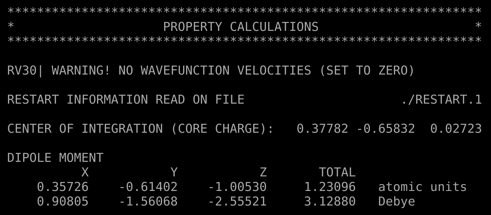
This calculation will be much faster than the previous one, and will produce different output files. In particular, the dipole.out file contain a CALCULATE DIPOLE MOMENT section, reporting the dipole moment along x,y,z axes and the total, both in atomic units and Debye.
This is what you should see:
System Preparation with GROMACS
Now we will move to the system preparation using classical (force field based) molecular dynamics. Create a folder where we are going to prepare the structure inputs and the topology for this tutorial:
mkdir ../2_system_prep
cd ../2_system_prep
Structure File
The structure file for acetone is provided in the data folder. Copy this file in the current folder:
cp ../../data/acetone.gro .
Structure files
.gro files contain molecular structure in Gromos87 format, in this case for the acetone molecule:
 Acetone molecule gas phase
 10
 1ACT     C1    1   5.041   5.034   5.035
 ...
 10.00000  10.00000  10.00000
The first line is the title (free string), the second line is the number of atoms (integer), and each of the following lines refers to one atom, reporting its residue number, residue name, atom name, atom number, position (x,y,z, in nm), and velocity (optional). The very last line contains the box vectors in x,y,z dimensions.
For more details see GROMACS documentation.
Topology
Also the topology files are provided in the data folder for this tutorial. Copy these files in the current folder:
cp ../../data/acetone.top .
cp ../../data/acetone.itp .
Topology files
.top files contain the topology for the system, i.e. the parameters used for the force field, in this case for the acetone molecule (that we will solvate). Topology files contain different sections:
; Include forcefield parameters
#include "amber03.ff/forcefield.itp"
#include "acetone.itp"

; Include SPC water topology
#include "amber03.ff/spc.itp"
Here different .itp files are included. Those files are where the parameters actually are stored. In this case we include parameters from the AMBER force field (#include "amber03.ff/forcefield.itp"), containing standard parameters for proteins and nucleic acids, prameters for acetone (#include "acetone.itp"), from the .itp file provided that we have just copied in the current folder, and parameters for water. Different water models exist (for more details on this topic see for this resource), and we choose to use the SPC rigid model, which is a three-site water model, i.e. contains three interaction points corresponding to the three atoms of the water molecule.
[ system ]
; Name
Acetone molecule
The [ system ] section, which needs to be placed after any other level, except the [ molecules ] one (here the previous sections are not shown, but are contained in the different .itp files). This section contains the name of the system (a string).
[ molecules ]
; Compound     #mols
ACT            1
The [ molecules ] section defines the total number of molecules i the system. Here, for the moment, we have only one acetone molecule. Each name present in this section must correspond to a name given with [ moleculetype ] previously in the topology (in our case, in the .itp files). The order of the blocks of molecule types and the numbers of molecules must match the coordinate file (acetone.gro in this case).
For more details see GROMACS documentation.
Solvation
After this preparatory step, we will now start to actually use GROMACS. Ensure that you either have GROMACS loaded into your coding environment.
We will solvate the acetone molecule, i.e. add water molecules to our structure. To do this, we can use the solvate command of GROMACS.
gmx solvate -cp acetone.gro -cs spc216.gro -p acetone.top -o solvated.gro -box 2.5 2.5 2.5
Where we have specified the water model (redundant here, since the spc216.gro model is the default one for the solvate command) and the size of the box, namely a cubic box of size 2.5nm.
The solvated structure is saved as solvated.gro, and the topology file has been updated. A backup file with the previous topology is saved as well, named #acetone.top.1#.
![]() Doublecheck the new topology: the last lines should appear as
Doublecheck the new topology: the last lines should appear as
ACT      1
SOL        506
with a single line per molecule type. If this is not the case and a single line is present after running the solvate command, i.e.
ACT 1SOL 506
edit the topology as explained aboove with one line per molecule type!
gmx solvate
The solvate command solvates a solute configuration in a box filled with solvent molecules. Different options can be used:
-cpstructure file for the solute, such as a protein-csstructure file for the solvent (wherespc216.grois the default one, i.e. SPC water model)-ptopology file for the system-boxbox size (x,y,z vectors) in nm
This command will produce a new structure file containing the solvated system, and will also update the topology file (keeping a backup version of the input topology). In particular, the [ molecules ] section of the topology will now contain
[ molecules ]
; Compound        #mols
ACT            1
SOL            506
Specifying that 506 solvent molecules, with molecule type SOL, which is defined in the water topology file that we already included in the main topology file.
For more details see GROMACS documentation.
Classical Equilibration
We are interested in studying the effects of the presence of water molecules on the dipole of acetone molecule, but the solvated system that we just created is based on the structure of acetone in vacuum. Hence, we need to equilibrate the system before continuing with QM/MM MD. In any case, the first step before running a QM/MM simulation is a classical force field-based molecular dynamics equilibration.
The equilibration we will perform is composed of two main steps:
Energy minimization on the initial structure which is needed to minimize the energy with the selected force field of the starting strucutre of the solvated system. This step will, for example, improve the orientation of hydrogen bonds.
Equilibration during which we will heat the system, using the minimized structure, by increasing temperature from 0K to 300K (room temperature).
Energy Minimization
Create a folder where we are going to perform the energy minimization step and copy the provided mini.mdp file, containing the parameters for the minimization:
mkdir ../3_mini
cd ../3_mini
cp ../../data/mini.mdp .
mini.mdp file
.mdp files contain parameters to set up a molecular dynamics run with a given system. We later process this file with the grompp command (explained later) to generate a binary .tpr file. The .mdp file parameters depend on the specific process and system so each time we move to a different MD process we’ll need a new .mdp input file (for example when we transition to QM/MM). Below we provide a sample .mdp file for an energy minimization run with comments following ; symbols:
    ; General MD parameters for an energy minimization process
    integrator    = steep    ; MD Algorithm selection (steep = steepest descent minimization).
    emtol         = 100.0    ; stop minimization when the maximum force < 100.0 kJ/mol/nm
    emstep        = 0.01     ; energy step size
    nsteps        = 50000    ; maximum number of (minimization) steps to perform

    ; Parameters describing how to find the neighbors of each atom and how to calculate their interactions
    nstlist        = 1       ; frequency to update the neighbor list and long range forces. Lowest possible value is 0 which equates to a list that is created and then never updated
    cutoff-scheme  = Verlet  ; type of cut-off scheme. `Verlet` generates a pair list with buffering
    ns_type        = grid    ; method to determine neighbor list (simple, grid)
    coulombtype    = PME     ; treatment of long range electrostatic interactions. This example shows a Particle-Mesh Ewald selection (`PME`). For more options see GROMACS documentation link below.
    rcoulomb       = 1.0     ; short-range electrostatic cut-off in nm
    rvdw           = 1.0     ; short-range Van der Waals cut-off in nm
    pbc            = xyz     ; periodic boundary conditions used in all directions (`xyz`). Other options could be `no` to ignore the box or `xy` to apply pbc to x and y directions only.
For more details see GROMACS documentation.
The .mdp files can be converted into binary files using the GROMACS preprocessor command grompp, which requires different inputs. Prior to running, make sure that ACT and SOL are on separate lines in molecules section of the acetone.top file.
gmx grompp -f mini.mdp -c ../2_system_prep/solvated.gro -p ../2_system_prep/acetone.top -o mini.tpr
grompp command
The grompp command converts our solvated.gro file from a molecular topology file into a binary file, mini.tpr, according to the parameters specified in the mini.mdp input file. Different options can be used:
-fread the MD parameter inputs from the.mdpfile-cstructure file in.groor.g96or.pdbor.brkor.entor.espor.tpr-ptopology file in.topformat-n[optional] index file in.ndxformat-ror-rb[optional] restraints in any of the formats possible with the-cflag, could even be the same file as provided for the-cflag-t[optional] trajectory in.trror.cptor.tngformat to read starting coordinates if needing to restart a process-e[optional] energy file in.edrformat to provide Nose-Hoover and/or Parrinello-Rahman coupling variables
Additionally, grompp uses a built-in preprocessor which can support the following keywords:
#ifdef VARIABLE
#ifndef VARIABLE
#else
#endif
#define VARIABLE
#undef VARIABLE
#include "filename"
#include <filename>
And these keywords can be enacted and changed in the associated .mdp file by including statements like:
define = -DVARIABLE1 -DVARIABLE2
include = -<file_path>
There are additional options to control the output files. For more details see GROMACS documentation.
Now that we generated the mini.tpr file, we are actually able to run the minimization using the mdrun command.
gmx mdrun -deffnm mini &
mdrun command
The `mdrun` launches molecular dynamics runs in GROMACS. Many different options can be used and just a few are listed below:
-deffnmuses the following string for all the file options (input, output, error, log, etc)-sportable xdr run input file in.tprformat-ooutput a full precisoin trajectory in a.trror.cptor.tngformat-cstructure file in.groor.g96or.pdbformat-ntompnumber of OpenMP threads per MPI rank
For more details see GROMACS documentation.
This prodecure will generate different output files. In particular, the progress of the minization can be monitored using the .log file, using the command
tail -f mini.log
When the minimization will be completed, a mesage will be printed in the log file, stating how many steps have been required to converge the minimization, together with other interesting quantities to look at, such as the potential energy of the final configuration and the maximum force (and the atom on which it acts).
The final configuration can be found in the mini.gro file, and will become the starting point for the heating phase.
Heating - Classical Equilibration
The next step is to thermalize the system classically and to adjust the pressure in the box to reach standard conditions. Create a folder where we are going to perform the heating step and copy there the heat.mdp input file provided. We need a new .mdp file because we are are performing a different type of simulation and therefore need different parameters.
mkdir ../4_heat
cd ../4_heat
cp ../../data/heat.mdp .
heat.mdp file
The heat.mdp requires information about the temperature and pressure control. You’ll see that we need to define more parameters than we did for the simple energy minimization process. Below we provide a sample .mdp file for a classical equilibration run with comments following ; symbols:
; Run parameters
integrator      = md          ; MD Algorithm selection (leap-frog integrator)
dt              = 0.002       ; time step in ps. Here we define a 2 fs time step
nsteps          = 100000      ; number of steps in the simulation. Here: 2 fs/step * 100000 steps = 200 ps

; Output control
nstxout         = 500         ; save coordinates every 1.0 ps
nstvout         = 500         ; save velocities every 1.0 ps
nstenergy       = 500         ; save energies every 1.0 ps
nstlog          = 500         ; update log file every 1.0 ps

; Bond parameters
continuation    = no          ; when turned on, this option specifies NOT to apply constraints to start or to reset shells.
                              ; This is useful to switch to `yes` for a re-run or an exact continuation.
                              ; Since this is our first dynamics run in the process we have this option set to `no` so that the constraints are applied at the start of the run.
constraint_algorithm  = lincs ; choice of constraint solver for any non-SETTLE holonomic constraints. Here we select a LINear Constraint Solver (lincs).
constraints     = all-bonds   ; which bonds are constrainted. `all bonds` means all bonds convert to constraints (even heavy atom-H bonds).
lincs_iter      = 1           ; max number of iterations for the lincs solver which controls the accuracy of LINCS
lincs_order     = 4           ; number of matrices in the expansion for the matrix inversion during constraint solving. This is also related to accuracy

; Neighbor searching
cutoff-scheme   = Verlet      ; type of cut-off scheme. `Verlet` generates a pair list with buffering
ns_type         = grid        ; method to determine neighbor list (simple, grid)
nstlist         = 10          ; frequency to update the neighbor list and long range forces. Lowest possible value is 0 which equates to a list that i is created and then never updated. This option is largely irrelevant with a Verlet cut-off scheme.
rcoulomb        = 1.2         ; short-range electrostatic cutoff in nm
rvdw            = 1.2         ; short-range van der Waals cutoff in nm

; Electrostatics
coulombtype     = PME         ; treatment of long range electrostatic interactions. This example shows a Particle-Mesh Ewald selection (`PME`). For more options see GROMACS documentation link below.
pme_order       = 4           ; order of PME interpolation. Here we define a cubic interpolation.
fourierspacing  = 0.16        ; grid spacing for FFT in nm. For optimizing the relative load of the particle-particle interactions and the mesh part of PME, it is useful to know that the accuracy of the electrostatics remains nearly constant when the Coulomb cut-off and the PME grid spacing are scaled by the same factor.

; Temperature coupling
tcoupl          = V-rescale   ; selection of thermostat/temperature control scheme. Here we select a modified Berendsen thermostat.
tc-grps         = System      ; define groups to couple to separate thermal baths. Here, with two coupling groups for system and solvent (basically everything else except the system) we can run a more accurate/efficient equilibration process.
tau_t           = 0.1         ; time constant for coupling with the bath in ps. A value of -1 specifies no coupling.
ref_t           = 300         ; reference temperature, one for each group defined, in K

; Pressure coupling
pcoupl          = Berendsen   ; selection of barostat/pressure control scheme. Here we select a modified Berendsen barostatting scheme.
pcoupltype      = isotropic   ; type or isotropy of pressure coupling. Here we employ a uniform scaling of box vectors with tau-p. When this option is selected a compressibility value and reference pressure value are required.
tau_p           = 2.0         ; time constant for pressure coupling, in ps
ref_p           = 1.0         ; reference pressure, in bar
compressibility = 4.5e-5      ; isothermal compressibility of water at your target conditions, bar^-1

; Periodic boundary conditions
pbc             = xyz         ; periodic boundary conditions used in all directions (`xyz`). Other options could be `no` to ignore the box or `xy` to apply pbc to x and y directions only.

; Dispersion correction
DispCorr        = EnerPres    ; dispersion corrections to account for the cut-off applied for vdw. Here `EnerPres` tells our system to apply long range disperssion corrections for both Energy and Pressure outputs.

; Velocity generation
gen_vel         = yes         ; generate velocities with a random seed according to a Maxwell distribution
gen_temp        = 300         ; temperature for the Maxwell distribution
gen_seed        = -1          ; generate a random seed. A `-1` value uses a pseudo random seed
For more details see GROMACS documentation.
As before, we first need to create the .tpr binary file using the GROMACS preprocessor command grompp, where the starting
gmx grompp -f heat.mdp -c ../3_mini/mini.gro -p ../2_system_prep/acetone.top -o heat.tpr
and then run the equilibration simulation:
gmx mdrun -deffnm heat &
As before, the progress of the heating phase can be monitored using the tail command
tail -f heat.log
and at the end a report will be printed to the file, and a heat.gro file containing the equilibrated configuration will be generated.
Selecting a thermostat
GROMACS provides several options for temperature control during a molecular dynamics simulation. You can add the option in the .mdp file with the keyword tcoupl followed by one of the options below:
-nono temperature control-nose-hooverthe Nose-Hoover thermostat defines an extended Lagrangian to manage the thermostat variables. Nose-Hoover chains are the typical choice for NVE production runs due to their stabiliy.-berendsenthe Berendsen thermostat adds a small coupling factor which moves the system towards a reference temperature. This is a “historical” thermostat mainly present to be able to reproduce previous simulations, but it is strongly recommend not to use it for new production runs-andersenthe Andersen thermostat randomizes velocities of some particles at each time step-andersen-massivethe Andersen massive thermostat randomizes velocities of some particles but not at each time step-v-rescaletemperature coupling using velocity rescaling with a stochastic term. This thermostat is similar to Berendsen coupling, but the stochastic term ensures that a proper canonical ensemble is generated.
We must define other thermostat variables in the .mdp file such as reference temperature (ref-t) and time constant for coupling (tau-t). For more details see GROMACS documentation:.
Equilibration Check
Is the system well equilibrated? One way to asses that is the GROMACS energy tool. This allows to monitor the behavior along the trajectory of the quantities you are interested in. Select the quantities you want to check using the corresponding number, and type a 0 to exit the command:
gmx energy -f heat.edr -o heat_check.xvg
for example, to look at total energy (11) and temperature (13), type:
> 11 13 0
This will perform a statistical analysis over all the steps stored in the .edr file and plot in particular the average and the estimated error on the terminal. You should obtain something similar to:
Statistics over 100001 steps [ 0.0000 through 200.0000 ps ], 2 data sets
All statistics are over 1001 points

Energy                      Average   Err.Est.       RMSD  Tot-Drift
-------------------------------------------------------------------------------
Total Energy               -17521.7        6.8    222.898   0.964539  (kJ/mol)
Temperature                 299.609       0.41    8.01493   0.616571  (K)
Check that the average temperature is close to 300K, or in general to the temperature you set as ref-t, without too large of fluctuations.
Note that the above command has also generated a heat_check.xvg file, which is helpful to plot and visually inspect data. This file is organized in columns based on the quantities selected before. In our case, the first column contains the time in ps (we asked GROMACS to store the energy every 500 steps, i.e. 1 ps using a timestep of 0.002 ps, setting nstenergy 500 in the heat.mdp file).
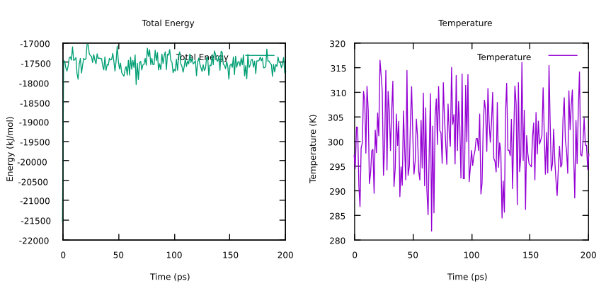
You can use any program to visualize this, in particular using gnuplot the commands needed to plot Total-Energy (column 2) and Temperature (column 3), are:
gnuplot
set multiplot layout 1, 2
set title "Total Energy"
set xlabel "Time (ps)"
set ylabel "Energy (kJ/mol)"
plot 'heat_check.xvg' u 1:2 w l lt 2 title "Total Energy"
set title "Temperature"
set xlabel "Time (ps)"
set ylabel "Temperature (K)"
plot 'heat_check.xvg' u 1:3 w l lt 1 title "Temperature"
Here you can see an example of the evolution of these two quantities during the heating phase. In particular, both energy and temperature should oscillate around fixed values, in particular equal to 300K (ref-t) for the temperature. These two plots, together with the average values and the errors estimated with the energy tool, confirm that the system is well equilibrated. We are now finally ready to run QM/MM MD!
QM/MM MD with MiMiC
Now that the preliminary steps are completed, and the system has been equilibrated at classical level, we are finally ready to run QM/MM MD! In particular, we want to run a QM/MM simulation in which the aceton molecule is treated quantum mechanically, while the surrounding water molecules are treated at classical MM level.
![]() All the files generated during the preliminary steps useful to start a QM/MM simulation are provided in the
All the files generated during the preliminary steps useful to start a QM/MM simulation are provided in the AcetoneTutorial/data/ folder.
![]() In case you skipped the first sections and you are starting the tutorial from this point, run this preliminary commands to download the corresponding git repository and create a
In case you skipped the first sections and you are starting the tutorial from this point, run this preliminary commands to download the corresponding git repository and create a solution folder, hence you will have the provided folders and files in the same locations.
curl https://gitlab.com/mimic-project/mimic-docs/-/archive/main/mimic-docs-main.tar.gz?path=docs/tutorials/AcetoneTutorial -o AcetoneTutorial.tar.gz
tar --strip-components=3 -zxvf AcetoneTutorial.tar.gz
cd AcetoneTutorial
mkdir solution
cd solution
You can now either copy your files a new folder inside the solution folder (if you have followed the tutorial so far), or use the ones provided (if you are starting the tutorial now, or you are not confident about the files you generated).
mkdir 5_mimic_prep
cd 5_mimic_prep
cp ../../data/acetone_equilibrated.gro ./heat.gro
cp ../../data/acetone_equilibrated.top ./acetone.top
cp ../../data/acetone.itp .
Input Preparation with MiMiCPy
MiMiC uses CPMD together with GROMACS in order to run a QM/MM simulation. The Python package MiMiCPy is the companion library to MiMiC in the preparation of QM/MM simulations. It comes with a set of command lines tools to prepare MiMiC input scripts. Additionally, plugins for PyMOL and VMD are also provided.
Instructions to install the MiMiCPy can be found in the Installation/MiMiCPy section.
Index file and GROMACS tpr
The CPMD input file and the GROMACS .tpr binary file have to be prepared at the same time, making sure that both CPMD and GROMACS receive the same QM atoms information. This can be easily achieved with the MiMiCPy package. As explained in the introduction, we assume you already installed mimicpy.
In particular, the MiMiCPy prepqm script allows the user to easily generate a CPMD input script (default name cpmd.inp) and a GROMACS index file (default name index.ndx). The latter can be used to generate the GROMACS .tpr file needed for the QM/MM simulation with MiMiC.
Run the MiMiCPy prepqm script:
mimicpy prepqm -top acetone.top -coords heat.gro
The command will open an interactive session with the following message printed out:
Some atom types had no atom number information.
They were guessed as follows:

+---------------------+
| Atom Type | Element |
+---------------------+
|     c     |    C    |
+---------------------+
|     c3    |    C    |
+---------------------+
|     o     |    O    |
+---------------------+
|     hc    |    H    |
+---------------------+
MiMiCPy requires the atomic element information for each atom to generate the CPMD input script. Some non-standard atom types in the GROMACS topology file do not contain this information. MiMiCPy guesses them based on the combination of atomic mass, name and type.
(! Always verify that the guessed atomic elements for each atom type are meaningful, as it is essential for CPMD to run correctly)
Handling non standard atomtypes with MiMiCPy
MiMiCPy guesses non-standard atom types based on the combination of atomic mass, name and type. The automatic behavior of guessing atomic elements can be toggled on or off using the -guess option. If False is passed and non-standard atoms are present, MiMiCPy will exit with an error message instead of attempting to guess the elements. If you are not satisfied with the element information guessed, a file containing the list of all non-standard atom types with the correct element information can be passed to mimicpy prepqm with the -nsa option. For example, if MiMiCPy guessed the wrong atomic number for atom type c3 and o, we could create a file called atomtypes.dat with the following text:
o O
c3 C
and pass it to MiMiCPy when running prepqm
mimicpy prepqm -top acetone.top -coords heat.gro -nsa atomtypes.dat
At this point, the user can provide instructions to add and/or deleted atoms to the QM region in an interactive session. The instructions specified after add correspond to the selection query that identifies the atoms to be added to the QM region. MiMiCPy provides a selection language similar to PyMOL and VMD for selecting QM atoms. In this case, we want to add the ACT molecule to the QM region with the following command:
> add resname is ACT
> q
MiMiCPy now generated the CPMD input script cpmd.inp and a GROMACS index file index.ndx. The latter contains the indeces of the QM atoms in the GROMACS topology, and needs to be used to generate the GROMACS .tpr file needed for the QM/MM simulation with MiMiC.
If you’d prefer, the same instruction add resname is ACT can be stored as a file sele.dat and passed to mimicpy prepqm for faster execution. In the case the selection is provided as input file:
cp ../../data/sele.dat .
In this case (not necessary now that you’ve alrready completed the prepqm step with the interactive session), the prepqm script can be run with an additional input -sele:
mimicpy prepqm -top acetone.top -coords heat.gro -sele sele.dat
As explained above, this command generates the CPMD input script cpmd.inp and a GROMACS index file index.ndx.
Selection query in MiMiCPy command
The syntax for the selection query involves the following general structure:
keyword logical_operator value
where keyword can include resname, resid, name, type, id, and mol. logical_operator can be is, not, >, <, >=, or <=.
Different selection queries can be joined by using and or or operators, and grouped with brackets, such as
add (resname is RES) and (name is x)
which will add atom named X of residue RES.
With the same selection syntax atoms can also be deleted from the QM region, using the delete command instead of add.
To check the current QM region, the view command can be used. When the desired QM atoms are selected, type q to exit.
A binary .tpr file can be generated using GROMACS preprocessor (gmx grompp), analogoulsy to what was is usually done with GROMACS (as done in the Classical Equilibration section. Copy the .mdp file provided and run GROMACS preprocessor, passing the index file just generated. It is important that the label for QMMM-groups matches the index file label (here qmatoms)!
cp ../../data/mimic.mdp .
gmx grompp -f mimic.mdp -c heat.gro -p acetone.top -o mimic.tpr -n index.ndx
The same coordinate and topology file used to run the earlier MiMiCPy command should be passed to gromacs grompp as well.
The two steps that we have just performed, i.e. generating an index file with MiMiCPy and using that to run the GROMACS preprocessor, can be combined in a single MiMiCPy command. In particular, if you selected the QM atoms in the sele.dat file, the mimic.mdp file can be passed to mimicpy prepqm command and this will automatically generate not only the index.ndx file, but also the mimic.tpr file.
![]() Before running the next command, make sure GROMACS has been sourced, i.e. is available on the command line. In particular, you may need to set the environment variable
Before running the next command, make sure GROMACS has been sourced, i.e. is available on the command line. In particular, you may need to set the environment variable GMXLIB with the following command, where the path to use the the one where the GROMACS share/gromacs folder is located
export GMXLIB='/path-to-gromacs-installation/share/gromacs/'
Now you can run mimicpy:
mimicpy prepqm -top acetone.top -coords heat.gro -sele sele.dat -mdp mimic.mdp -gmx gmx -tpr mimic.tpr
With this command, MiMiCPy would generate not only the cpmd.inp and index.ndx files as before, but also mimic.tpr using gmx grompp, like the GROMACS command we just ran. Note that in order to excute this MiMiCPy command you will need to have correctly sourced GROMACS and loaded all necessary modules as this command includes a call to GROMACS to perform the grompp command.
CPMD input
Together with the index.ndx and/or mimic.tpr file, MiMiCPy generated also the CPMD input script cpmd.inp. This is a barebones CPMD input file, containing the most essential commands to run a MiMiC simulation.
MiMiC input for CPMD command
A CPMD input file for a QM/MM simulation is similar to the CPMD input file for a standard QM calculation that has been previously described (Introduction section: Dipole Moment in Vacuum with CPMD). However, there are some main differences that should always be taken into account for the new QM/MM interface of CPMD:
In the
&CPMDsection the keywordMIMICneeds to be addedA new
&MIMICsection, is mandatory. This section is the output from the MiMiCPy preprocessor, the 3 required keywordsPATHS,BOXandOVERLAPSare provided. In this section, also other keywords can be added. The most relevant keywords for the&MIMICsection are:PATHS, the number of the additional layers beyond the QM one treated by CPMD. In the case of QM/MM, this is1. In the following lines, for each layer the absolute path where the corresponding files are stored has to be specified (in our case the path where the GROMACS.tprfile is located). Always check that this path is consistent and is not indented - otherwise the simulation will get crash!
BOX, the size of the classical box, in a.u.OVERLAPS, i.e. how many (first line) and which are the atoms (following lines) from one of the codes that should be treated by another one. In our case in this section the QM atom needs to be specified. The format for the lines specifying the overlapping atoms is a sequence of four numbers representing: the code (CPMD = 1, GROMACS = 2), the atom ID, the cpde ID that has to treat it, and the atom ID in that code.LONG-RANGE COUPLING, which turns on (if present) long-ranged electrostatic coupling to minimize the computational cost of the simulation. Interactions with MM atoms withinCUTOFF DISTANCE(20in this case) will be treated using explicit Coulomb potential. For atoms that are outside the cutoff, a multipolar expansion of the electrostatic potential of an electronic grid will be used.FRAGMENT SORTING ATOM-WISE UPDATE, which specifies the sorting frequency, i.e. the number of steps between two consecutive sorting of the atoms into the short and the long-ranged groups (100in this case).MULTIPOLE ORDER, which dictates the order at which the multipolar expansion is trucated (3in this case).
In the
&ATOMSsection, the QM atoms has to be specified as in the full QM calculations.The keyword
ANGSTROMin the&SYSTEMsection cannot be used. Lengths have to be expressed in a.u.The option
ABSOLUTEin the keywordCELLcannot be used. The correct syntax for the size of an orthorhombic box A x B x C isA B/A C/A 0 0 0The QM system in a QM/MM calculation can only be dealt as isolated system, i.e. without explicit PBC since there is the MM environment all round it. Even though the option
ISOLATED SYSTEM(or0) is used for theSYMMETRYkeyword, the calculation is, in fact, still done in a periodic cell: we are still using a plane wave basis set to expand the wavefunction of the QM part. Since the acetone molecule has a dipole moment, we have to take care of the long-range interactions between periodic images and there are methods (activated with the keywordPOISSON SOLVERin the&SYSTEMsection) implemented in CPMD to compensate for this effect. In particular,TUCKERMANPoisson solver is used, since it has been proven to be the most effective one with typical systems studied in biology. Decoupling of the electrostatic images in the Poisson solver requires increasing the box size over the dimension of the molecule: practical experience shows that 3-3.5 Å between the outmost atoms and the box walls is usually sufficient for typical biological systems.
Details of the CPMD input to perform QM/MM calculations with MiMiC are described in the above drop-down menu. In particular, few things need to be noted/fixed:
The path specified in the
PATHSkeyword of the&MIMICsection refers to the path of the directory from which GROMACS will be run, i.e. where themimic.tprfile is located. By default, MiMiCPy uses the current directory. Alternatively, a path can be specified with the-pathoption when runningmimicpy prepqm. Always check that this path is consistent and is not indented - otherwise the simulation will get crash!The size of the QM region is specified in the
CELLkeyword in the&SYSTEMsection. The cell size cannot be written in theABSOLUTEformat, and the correct syntax for the size of an orthorhombic boxA x B x Cis
CELL A B/A C/A 0 0 0
where0 0 0refer to the cosines of the angles between the vector, i.e. perpendicular vectors in this case. By default, MiMiCPy writes a cell size exactly bounding the QM region. This is often not enough to contain the plane waves of the QM region. For this reason, a padding needs to be added: this can be done using the-padoption when runningmimicpy prepqm, i.e. an additional distance between the QM atoms and the walls of the QM box (in nm). A standard value for the Poisson solver is 3-3.5 Å , but in general the question of the right padding should be considered and chosen wisely depending on the system under study. MiMiCPy adds this on both sides in each direction; therefore, with a-padof 0.3, a value of 0.7 nm is actually added in each direction to the size of the QM systemThe charge of the QM region is specified in the
CHARGEkeyword in the&SYSTEMsection. This is calculated by MiMiCPy by summing the MM charges read from the force field data. This is usually enough, but it may need to be cross checked. Alternatively, a charge value to be written in the output can be specified using the-qoption when runningmimicpy prepqm.The QM atoms are specified in the
&ATOMSsection. Default values are written by MiMiCPy, but pseudopotential information needs to be adapted. This can be done by hand or passed a filepp_info.dat(provided) to the-ppoption of mimicpy prepqm. This file should contains information like the pseuodopotential filenames for a specific atom, the same for the link atom version and other labels like LMAX and LOC.
Keep the LMAXvalues consistent with what we used for the dipole moment calculation in vacuum, namelySforHandPforCandO. By default, all these have been set toSby the preprocessor if the-ppoption is not used (see below).
The extra sections not in cpmd.inp file outputted by MiMiCPy can be added in by hand. A more efficient way is to store all the extra parameters in a separate template file template.inp (provided). In the example provided, these are the parameters required for a full MiMiC simulated annealing (excluding the parameters in &ATOMS and &MIMIC sections outputted by mimicpy prepqm). Other options can be specified, they can be listed by typing mimicpy prepqm --help.
You can edit manually the cpmd.inp file, or invoke MiMiCPy again, this time passing all the option that we mentioned above: the template.inp file via the -inp option to provide a template for the generation of the complete input file, the -pad option, to properly define the size of the QM region. We now use the same procedure explained in the previous section, passing also the the selection of the QM atoms as input (using the sele.dat file), and we will also use the -gmx option, to directly invoke the grompp GROMACS preprocessor.
![]() Before running the next command, make sure GROMACS has been sourced, i.e. is available on the command line. In particular, you may need to set the environment variable
Before running the next command, make sure GROMACS has been sourced, i.e. is available on the command line. In particular, you may need to set the environment variable GMXLIB with the following command, where the path to use the the one where the GROMACS share/gromacs folder is located
export GMXLIB='/path-to-gromacs-installation/share/gromacs/'
Now you can run:
cp ../../data/sele.dat .
cp ../../data/pp_info.dat .
cp ../../data/template.inp .
mimicpy prepqm -top acetone.top -coords heat.gro -sele sele.dat -inp template.inp  -pp pp_info.dat -pad 0.35 -out annealing.inp -mdp mimic.mdp -gmx gmx -tpr mimic.tpr
With the last command, we overwrote the index.ndx and the mimi.tpr files previously generated. This last command shows you how you can easily generate those two files, together with a complete CPMD input for MiMiC, using MiMiCPy. In particular, this time MiMiCPy inserts the &ATOMS section, etc. into template.inp, generating the annealing.inp CPMD input file (whose name has been specified with the option -out). This is a full CPMD input file ready to be used for running MiMiC.
QM/MM calculations
In the previous sections, we obtained the equilibrated coordinates at room conditions using classical MD. This will be the starting point for a QM/MM simulation. However, we first need to equilibrate the system at QM/MM level since the two levels of theory are different. Therefore, it is necessary to firstly optimize the geometry of the system. Once we have a QM/MM minimized structure, we can heat the system to room temperature and run a QM/MM MD simulation.
Annealing
A minimal energy structure at QM/MM level can be obtained with a simulated annealing (this is the reason of the keyword ANNEALING IONS in the input file), i.e. we run a Born-Oppenheimer MD where gradually removing kinetic energy from the nuclei by multiplying velocities with a factor (set to 0.95 in our input, so 5% of the kinetic energy will be removed at each step). Create a new folder where we will perform the annealing and copy all the files needed for the simulation:
mkdir ../6_annealing
cd ../6_annealing
cp ../5_mimic_prep/mimic.tpr .
cp ../5_mimic_prep/annealing.inp .
![]() Update the path in the
Update the path in the PATH keyword in the &MIMIC section - no white spaces!
CPMD input for annealing command
The &CPMD section contains few keyword which have not been explained in detail yet:
MOLECULAR DYNAMICS BO, to perform a molecular dynamics run.BOstands for a Born-Oppenheimer type of MD. An alternative option isCP, which stands for a Car-Parrinello type MD.ANNEALING IONS, specifies to perform a simulated annealing simulation, where kinetic energy is gradually removed from the nuclei by multiplying velocities with a factor specified in the following line (0.99here, so 1% of the kinetic energy removed at each step).NEW CONSTRAINTS, which swtiches on the new constraint solver specifically designed for the MiMiC interfaceTEMPERATURE, the initial temperature for the atoms (in Kelvin), specified in the following line (300in this case). Here we choose the temperature at which we equilibrated the system at force field level.TIMESTEP, time step (in a.u.), specified in the following line (10in this case). The choice of the timestep is crucial to have a stable simulation, and at the same time to optimize the time for the computation. For BO MD, a time step of 10 a.u. (~ 0.24 fs) is usual.MAXSTEP, maximum number of steps for MD to be performed, specified in the following line.TRAJECTORY SAMPLE, the frequency at which to save atomic positions, velocities and optionally forces. It is specified with a number, corresponding to the number of steps, specified in the following line. If this is set to0, noTRAJECTORYfile will be written.STORE, the fequency at which to update theRESTARTfile. It is specified with a number, corresponding to the number of steps, specified in the following line.RESTFILE, the number of distinctRESTARTfiles generated during CPMD runs, specified in the next line.
A QM/MM simulation with the MiMiC interface will require running at the same time two different (parallel) processes, one for CPMD and one for GROMACS. The user is totally free to choose the best partitioning for the nodes/cores at one’s own disposal, but in this tutorial we require two cores for CPMD and one core for GROMACS: in the largest majority of the cases one core for GROMACS is enough. Run the annealing (all command as one line), making sure to specify the correct path to the AcetoneTutorial folder, instead of path-to-tutorial-folder, to provide CPMD the pseudopotentials.
To run CPMD, you need to provide pseudopotentials as second input in the cpmd.x command (see below). Pseudopotentials are not distributed with CPMD, so do not forget to download them either from the CPMD website or your favourite pseudopotential repository. The pseudopotentials needed for this tutorial are provided in the AcetoneTutorial/data/pseudo repository.
First we set all the OpenMP threads to 1 to ensure each core is excuting effectively. In this run of MiMiC, we will use three cores, 2 for CPMD and 1 for GROMACS.
export OMP_NUM_THREADS=1
mpirun -n 2 cpmd.x annealing.inp path-to-tutorial-folder/AcetoneTutorial/data/pseudo > annealing.out : -n 1 gmx mdrun -deffnm mimic -ntomp 1 &
While the simulation runs you can monitor the decreasing temperature (third column of the ENERGIES file):
tail -f ENERGIES
The calculation will perform 300 steps (MAXSTEP in the annealing.inp file). These should be enough to reach a low temperature, about 1-2K. Once the annealing is compelted, the last configuration will be stored in the RESTART.1 file (the last restart file written is anyway specified in the LATEST file). Wait until CPMD finishes writing the file and then verify that CPMD and GROMACS processes are stopped.
The annealing.out file reports some new sections with respect to what we have seen in the Dipole Moment in Vacuum with CPMD section (which was a pure QM calculation):
The energy report shows the different energetic contributions, for example:
(K+E1+L+N+X+MM+QM/MM)  TOTAL ENERGY =          -44.53592240 A.U.
 (K+E1+L+N+X)        TOTAL QM ENERGY =          -36.46982014 A.U.
 (MM)                TOTAL MM ENERGY =           -8.02852010 A.U.
 (QM/MM)          TOTAL QM/MM ENERGY =           -0.03758217 A.U.
 (K)                  KINETIC ENERGY =           28.12240741 A.U.
 (E1=A-S+R)     ELECTROSTATIC ENERGY =          -27.50067179 A.U.
 (S)                           ESELF =           29.92067103 A.U.
 (R)                             ESR =            1.78558591 A.U.
 (L)    LOCAL PSEUDOPOTENTIAL ENERGY =          -29.86421972 A.U.
 (N)      N-L PSEUDOPOTENTIAL ENERGY =            3.61298065 A.U.
 (X)     EXCHANGE-CORRELATION ENERGY =          -10.84031668 A.U.
          GRADIENT CORRECTION ENERGY =           -0.57543727 A.U.
After the force initialization section, BO MD begins: for each MD step, the wavefunction is re-converged. The MD step number is indicated as
NFI(number of finite iterations), and for MD each step different quantities are reported: temperature, calculated as the kinetic energy divided by the degrees of freedom (TEMPP), quantum DFT Kohn-Sham electron energy, equivalent to the potential energy in classical MD (EKS), total energy in a classical MD (ECLASSIC), mean squared displacement of the atoms from the initial coordinates (DIS), and the time took to calculate this step (TCPU). Since in BO MD the wavefunction is re-converged, for each step information about the convergence are reported.NFI TEMPP EKS ECLASSIC DIS TCPU 1 297.1 -44.53592 -43.09507 0.844E-04 16.34 INFR GEMAX ETOT DETOT TCPU 1 8.907E-04 -36.507197 0.000E+00 3.02 2 4.218E-04 -36.507428 -2.304E-04 1.32 3 2.169E-04 -36.507444 -1.607E-05 1.34 4 1.922E-04 -36.507447 -3.256E-06 1.37 5 9.735E-05 -36.507447 -5.238E-07 1.36 6 3.486E-05 -36.507448 -1.715E-07 1.40 7 2.119E-05 -36.507448 -9.343E-08 1.41 8 1.248E-05 -36.507448 -5.398E-08 1.39 9 5.057E-06 -36.507448 -2.455E-08 1.46 2 294.2 -44.53611 -43.10943 0.172E-03 82.96 INFR GEMAX ETOT DETOT TCPU 1 8.942E-04 -36.507225 0.000E+00 3.02 2 4.189E-04 -36.507455 -2.304E-04 1.34 3 2.159E-04 -36.507472 -1.613E-05 1.35 4 1.981E-04 -36.507475 -3.273E-06 1.33 5 9.894E-05 -36.507475 -5.344E-07 1.40 6 3.474E-05 -36.507476 -1.739E-07 1.42 7 2.159E-05 -36.507476 -9.483E-08 1.10 8 1.275E-05 -36.507476 -5.612E-08 1.12 9 5.119E-06 -36.507476 -2.584E-08 1.09 ...
When the simulation is completed (due to the maximum number of steps/computational time reached or “soft”
EXITmessage received), a summary of averages and root mean squared deviations for some of the monitored quantities is reported. This is useful to detect unwanted energy drifts or too large fluctuations in the simulation:RESTART INFORMATION WRITTEN ON FILE ./RESTART.1 SUBSYSTEM 1 SR ATOMS PER PROCESS GROUP 493 SUBSYSTEM 1 SR ATOMS PER PROCESS 247 SUBSYSTEM 1 LR ATOMS PER PROCESS GROUP 1035 SUBSYSTEM 1 LR ATOMS PER PROCESS 518 **************************************************************** * AVERAGED QUANTITIES * **************************************************************** MEAN VALUE <x> DEVIATION <x^2>-<x>^2 IONIC TEMPERATURE 26.38 46.0235 DENSITY FUNCTIONAL ENERGY -45.672099 0.417524 CLASSICAL ENERGY -45.544157 0.614735 NOSE ENERGY ELECTRONS 0.000000 0.00000 NOSE ENERGY IONS 0.000000 0.00000 ENERGY OF CONSTRAINTS 0.000000 0.00000 ENERGY OF RESTRAINTS 0.000000 0.00000 BOGOLIUBOV CORRECTION 0.000000 0.00000 ION DISPLACEMENT 1.27023 0.844647 CPU TIME 35.9728
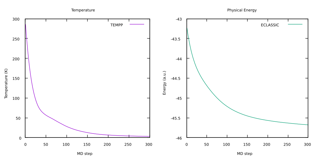
To have a visual check that the annealing proceeded as expected, you can have a look at the temperature and the physical energy to check they correctly stabilized. You can use any program to visualize this, in particular using
gnuplotthe commands needed to plotTEMPP(column3) andECLASSIC(column5), are:gnuplotset multiplot layout 1, 2 set title "Temperature" set xlabel "MD step" set ylabel "Temperature (K)" plot 'ENERGIES' u 1:3 w l lt 1 title "TEMPP" set title "Physical Energy" set xlabel "MD step" set ylabel "Energy (a.u.)" plot 'ENERGIES' u 1:5 w l lt 2 title "ECLASSIC"
Here you can see an example of the evolution of these two quantities during the test:
Test - NVE MD
In general, it is a good idea to verify that the final configuration obtained after the annealing is a physically ‘reasonable’ minimum energy configuration and that the BO MD has not brought the system in a very improbable configuration. A good test is to run a simulation in an NVE ensemble monitoring temperature (TEMPP) and physical energy (ECLASSIC): if after some steps these two quantities stabilize, then it is possible to be confident that the RESTART.1 file previously obtained contains a good minimum energy structure. On the other hand, if energy and/or temperature continuously increase, that means that a good structure has not yet been obtained, and another annealing procedure is required, usually starting from a different configuration (for example, after heating the system at 300 K in order to move the system away from that “wrong” energy potential basin), or changing the annealing parameters (for example the annealing factor in ANNEALING IONS).
The test can be performed by the following procedure:
Create a new folder and copy in it all the files needed (we will modify the input file used for the annealing):
mkdir ../7_test
cd ../7_test
cp ../6_annealing/mimic.tpr .
cp ../6_annealing/RESTART.1 ./RESTART
cp ../6_annealing/annealing.inp ./test.inp
Modify
test.inpfile so that the&CPMDsection appears as:&CPMD RESTART COORDINATES VELOCITIES WAVEFUNCTION MIMIC MOLECULAR DYNAMICS BO NEW CONSTRAINTS ISOLATED MOLECULE TIMESTEP 10.0 MAXSTEP 1000 TRAJECTORY SAMPLE 0 &END
![]() Update the path in the
Update the path in the PATH keyword in the &MIMIC section - no white spaces!
Run the test
mpirun -n 2 cpmd.x test.inp path-to-tutorial-folder/AcetoneTutorial/data/pseudo > test.out : -n 1 gmx mdrun -deffnm mimic -ntomp 1 &
Monitor the simulation:
tail -f ENERGIES
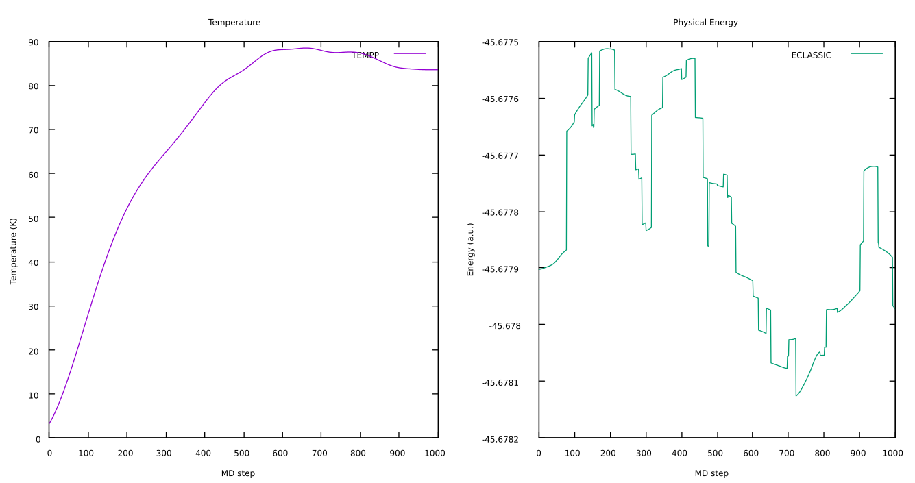
When the simulation is completed, you can have a look at the temperature and the physical energy to check they correctly stabilized. You can use any program to visualize this, in particular using
gnuplotthe commands needed to plotTEMPP(column3) andECLASSIC(column5), are:gnuplotset multiplot layout 1, 2 set title "Temperature" set xlabel "MD step" set ylabel "Temperature (K)" plot 'ENERGIES_1000' u 1:3 w l lt 1 title "TEMPP" set title "Physical Energy" set xlabel "MD step" set ylabel "Energy (a.u.)" plot 'ENERGIES_1000' u 1:5 w l lt 2 title "ECLASSIC"
Here you can see an example of the evolution of these two quantities during the test:
Heating
If the test is successful (or if you skipped it), we can come back to the configuration obtained by the annealing procedure and start heating the system up to the room temperature. One way to do this is to increase the target temperature of a thermostat (coupled to the system) linearly at each step by performing a usual BO MD. A simple Berendsen-type thermostat can be used in the heating phase: it does not fully preserve the correct canonical ensemble but we are not interested to this feature at this stage, while it is numerically fast and more stable than alternative algorithms.
You can heat the system by performing the following procedure:
Create a new folder and copy in it all the files needed (we will modify the input file used for the annealing):
mkdir ../8_heating
cd ../8_heating
cp ../6_annealing/mimic.tpr .
cp ../6_annealing/RESTART.1 ./RESTART
cp ../6_annealing/annealing.inp ./heating.inp
Modify
heating.inpfile so that the&CPMDsection appears as:&CPMD RESTART COORDINATES VELOCITIES WAVEFUNCTION MIMIC MOLECULAR DYNAMICS BO NEW CONSTRAINTS ISOLATED MOLECULE TEMPERATURE RAMP T_init 340.0 20 BERENDSEN IONS T_init 5000 TIMESTEP 10.0 MAXSTEP 1500 TRAJECTORY SAMPLE 1 &END
Update the path in the PATHkeyword in the&MIMICsection - no white spaces! Modify the T_initvalue in the input file: With respect to the input file used to perform the test, two additional keywords are added in the&CPMDsection: 1.TEMPERATUREwith the optionRAMP, where 3 numbers have to be specified on the line below the keyword: initial temperature (T_init, in K), target temperature (in K) and the ramping speed (in K per atomic time unit, to get the change per time step you have to multiply it with the value ofTIMESTEP). In particular, we set a target temperature slightly higher than our real target of 300 K, since the thermostat may require a long time before actually reaching the target temperature specified. 2.BERENDSENwith the optionIONS, where 2 numbers have to be specified on the line below the keyword: the target temperature for the termostat, which in our case is the initial one (T_init) and the time constant τ of the thermostat (in a.u.). The suggested value of 5000 a.u., corresponding to ~0.12 ps, is a reasonable value for the system.
The value ofT_initcorresponds to the final temperature of the annealing procedure, from which we are starting the heating. You can read it from theENERGIESfile generated in the annealing (third column) using the commandtail -1 ../6_annealing/ENERGIES, and set it accordingly in theheating.inpfile.Run the heating
mpirun -n 2 cpmd.x heating.inp path-to-tutorial-folder/AcetoneTutorial/data/pseudo > heating.out : -n 1 gmx mdrun -deffnm mimic -ntomp 1 &
Monitor the temperature during the simulation (third column):
tail -f ENERGIES
If the desired temperature is not reached at the end of the simulation, you can continue the heating adding two keywords in the
&CPMDsection in theRESTARTline ofheating.inp:LATEST, which ensures to use the lastest writtenRESTARTfile (whose name is contained in theLATESTfile)ACCUMULATORS, which ensures that new energy data and trajectory will be appended to your existing files. Run the job in the same working directory as before.
RESTART COORDINATES VELOCITIES WAVEFUNCTION LATEST ACCUMULATORS
When the simulation is completed, you can have a look at how the different quantities evolved during the heating phase. In particular, you can check how the temperature rises. You can use any program to visualize this, in particular using
gnuplotthe commands needed to plotTEMPP(column3) are:gnuplotset title "Temperature" set xlabel "MD step" set ylabel "Temperature (K)" plot 'ENERGIES' u 1:3 w l lt 1 title "TEMPP"
Here you can see an example of the rise in temperature during the heating. In particular, to obtain this plot we run a longer heating than the MAXSTEP we set previously, and we had to to restart it from time to time to be able to reach the desired temperature of 300K (as explained above):
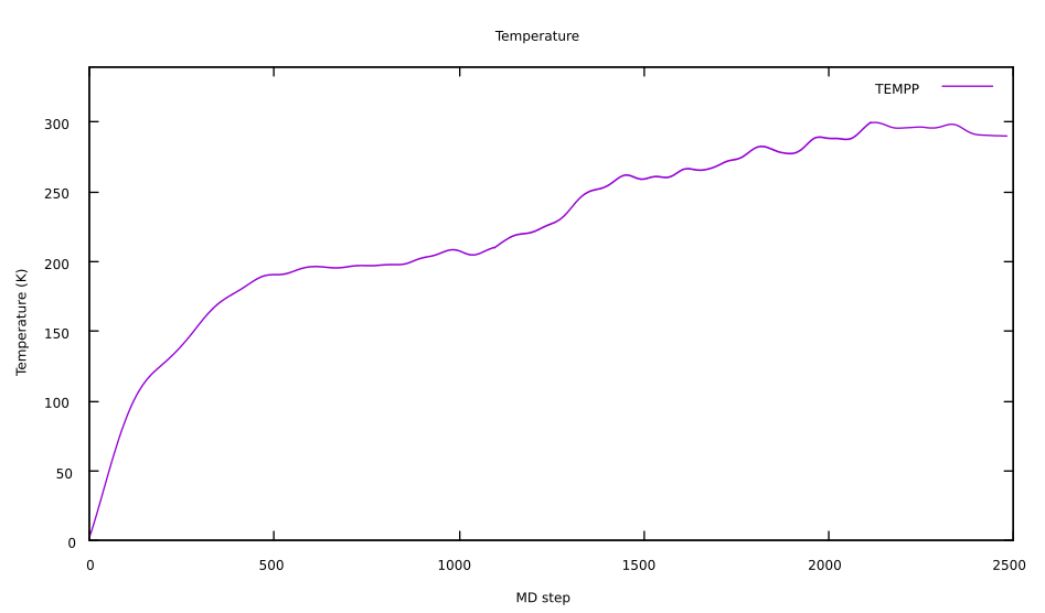
Note that the heating phase can be challenging: it is not always easy to get the temperature to stabilize to the desired value. The temperature specified in the RAMP will be eventually reached, but it may require a large amount of time, i.e. many more steps than the ones performed. What you can do in practice, if your system seems to be stabilized at a lower temperature than desired, is to restart the heating procedure from that intermediate point. You will then set the temperature for that configuration as T_init, and you can try to set a higher target temperature or a faster ramping speed.
Anyway, even if to run your own system you will of course need to compelte the heating phase, for this tutorial we sugget to move to the next section even if you did not manage to obtain a well equilibrated configuration at QM/MM level: we will provide one for you, so you can see also how to start a production run.
Production Run
Now that the system is well equilibrated, we are finally ready to run a QM/MM MD at room conditions.
You can run the production by performing the following procedure:
Create a new folder and copy in it all the files needed (we will modify the input file used for the heating):
mkdir ../9_production
cd ../9_production
cp ../8_heating/mimic.tpr .
cp ../8_heating/heating.inp ./prod.inp
cp ../8_heating/RESTART.1 ./RESTART
Modify
prod.inpfile so that the&CPMDsection appears as:&CPMD RESTART COORDINATES VELOCITIES WAVEFUNCTION GEOFILE MIMIC MOLECULAR DYNAMICS BO DIPOLE DYNAMICS NEW CONSTRAINTS ISOLATED MOLECULE DIPOLE DYNAMICS NOSE IONS 300 4000 TIMESTEP 10.0 MAXSTEP 1000 TRAJECTORY SAMPLE 100 STORE 100 RESTFILE 10 &END
Update the path in the PATHkeyword in the&MIMICsection - no white spaces!With respect to the input file used to perform the heating, we made some modifications:
The
GEOFILEoption has been added to theRESTARTkeywod. To perform the restart, this option will read old ionic positions and velocities from the fileGEOMETRY. Note that aRESTARTfile need to be present as well, to read informations about the system not present in the geometry file, such as the atom elements.The keywords
DIPOLE DYNAMICShave been added which captures dipole information during the production run everyNSTEPiteration in MD and saves it in an output file namedDIPOLE. TheNSTEPvalue is read from the next line if the keywordSAMPLEis present. But without this keyword and value, the default is1(every time step). Here we simply capture the dipole information at everystep. We will use the data stored in theDIPOLEfile in Dipole Calculation - method 1 section.BERENDSENthermostat for ions has been replaced withNOSE, corresponding with Nose-Hoover chains. As mentioned before, Berendsen a fast and stable thermostat, but does not properly samples the canonical ensemble. On the other hand, Nose-Hoover preserves the Maxwell distribution of the velocities and allows sampling the correct canonical ensemble, providing a NVT ensemble for a system in equilibrium. After theNOSE IONSkeyword, 2 numbers are specified: the target temperature for the termostat, which in our case is 300 K, and the thermostat frequency in cm-1, here 4000 cm-1. Concerning the choice of the thermostat frequency, at which the energy transfer from/to the thermostat happens, it is important not to select a resonance vibrational frequency of your system.The
MAXSTEPhas been increased to 10000 steps. Considering the timestep of choise (10 a.u.), this corresponds to a total simulation time of 100000 a.u., i.e. ~2.4 ps.The trajectory is stored every 100 steps (
TRAJECTORY SAMPLEoption), and during the simulation 10 restart files will be saved. This is selected choosing to update theRESTARTfile every 1000 steps (STOREoptions), and saving 10 distinctRESTARTfiles (RESTFILEoption). In this way, a sequence of filesRESTART.1,RESTART.2, …,RESTART.10will be produced during the dynamics. We will calculate the dipole moment of the acetone molecule for each of these configurations.
We want to start the production from a reasonably heated configuration. This can be done extracting the coordinates and velocities of a step of choice, where the temperature has reached the desired value. We will save this information in a
GEOMETRYfile, which will be used as starting point thanks to theGEOFILEoption we added to theRESTARTkeywod.
![]() Even in case you did not manage to obtain a well-equilibrated structure and you will use the
Even in case you did not manage to obtain a well-equilibrated structure and you will use the GEOMETRY file that we provide as starting point for the production (instructions below) it is useful to read the process described here to extract a GEOMETRY file from a TRAJECTROY since you will be likely perform this step when working with MiMiC with your systems.
We provide a useful script to do that, called geofile_extract.py, even if this can in principle be easily done manually from the TRAJECTORY file (but it is not so practical with large systems). In order to extract the coordinates and velocities, we need to choose a step at which doing it. We can do it using the ENERGIES file produced during the heating process. It is important to keep in mind that how often coordinates and velocities have been stored. In our case, we set TRAJECTORY SAMPLE 1, i.e. we stored coordinates and velocities each steps, so we are sure every step we see in the ENERGIES file will have a corresponding set of positions and velocities in the TRAJECTORY file (but this may not be the case). Inspect the ENERGIES file of the heating phase and select a step number (first column) where the temperature (third column) is aroud 300K
vi ../8_heating/ENERGIES
You will see something similar to
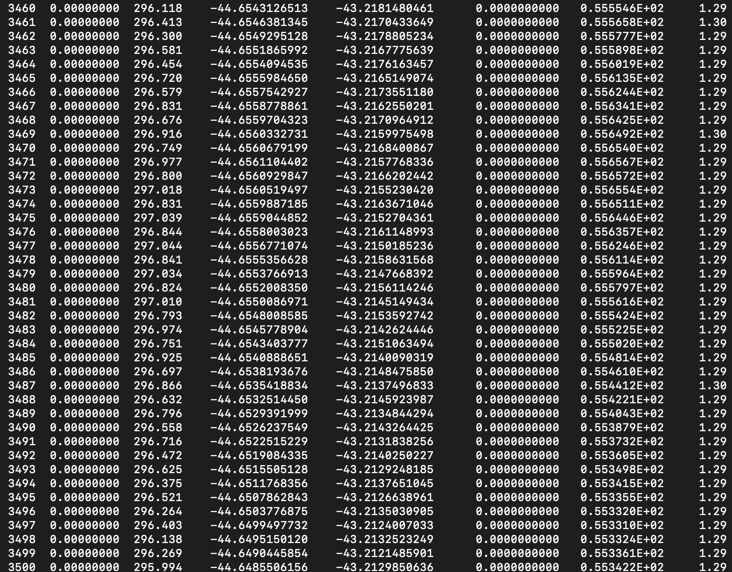
In this example, step 3477 seems a good choice as it is near 300K and shows stability in that range for a while. You could manually extract the coordinates and the TRAJECTORY file, and convert it in the GEOMETRY format. Otherwise, you can use the geofile_extract.py from the MiMiC Helper Script GitLab folder to extract the corresponding geometry.
wget https://gitlab.com/mimic-project/mimic_helper/-/raw/main/scripts/geofile_extract.py
python3 geofile_extract.py ../8_heating/TRAJECTORY ../8_heating/ENERGIES XXX
This will extract step XXX (which we would fill in as 3477 in our example) from the TRAJECTORY file, and check the corresponding temperature in the ENERGIES file. You will see in the ouput information about the temperature of the step selected, and the location of the corresponding geometry file.
This will generate a geometry file GEO_TTTK, where TTT is the temperature of the configuration. Copy the extracted geometry file, renaming it GEOMETRY, in the production run folder to use it as starting point for the production run
cp ../8_heating/GEO_TTTK ./GEOMETRY
In case you did not manage to obtain a well-equilibrated configuration at QM/MM level, you can start the production run using the
GEOMETRYprovided. Copy that in the current folder with the following commandcp ../../data/GEO_295K ./GEOMETRY
Now we have all the elements to run the production
mpirun -n 2 cpmd.x prod.inp path-to-tutorial-folder/AcetoneTutorial/data/pseudo > prod.out : -n 1 gmx mdrun -deffnm mimic -ntomp 1 &
You can monitor different quantities of interest during the production run, for example the temperature (
TEMPP, third column) and the physical energy (ECLASSIC, fifth column) of the system:tail -f ENERGIES
When the simulation is completed, you can have a look at how these two quantities evolved during the production phase. You can use any program to visualize this, in particular using
gnuplotthe commands needed to plotTEMPP(column3) are:TEMPP(column3) andECLASSIC(column5), are:gnuplotset multiplot layout 1, 2 set title "Temperature" set xlabel "MD step" set ylabel "Temperature (K)" plot 'ENERGIES' u 1:3 w l lt 1 title "TEMPP" set title "Physical Energy" set xlabel "MD step" set ylabel "Energy (a.u.)" plot 'ENERGIES' u 1:5 w l lt 2 title "ECLASSIC"
Here you can see an example of the evolution of these two quantities over the first 5000 steps of the production phase:
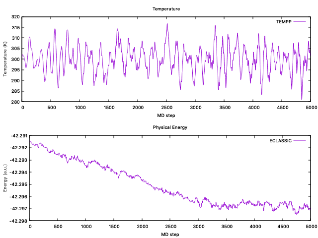
A very good practice when you perform a simulation is to look at your trajectory through some visualization tool. This in particular can be extremely helpful when you notice some strange behavior of some physical quantity: the most of the problems are immediately identified by visual inspection. To visualize a the trajectory you can for example use VMD. There are several options to do so:
By setting the option
TRAJECTORY XYZin the&CPMDsection the output fileTRAJEC.xyzis produced. This can be directly loaded into VMDvmd TRAJEC.xyz
In principle, all the information needed by VMD are present in two distinct files: the
GEOMETRY.xyzfile contains the information about the atom types, and theTRAJECTORYfile contains the cordinates at different timesteps. You can load theGEOMETRY.xyzfile in VMD and input in it theTRAJECTORY.vmd GEOMETRY.xyz
Then from the VMD menu right click on the
GEOMETRY.xyzmolecule, selectLoad Data Into Moleculeand load theTRAJECTORYfile, selectingCPMDin theDetermine file typedropdown menu. Be aware that in this way the first frame will be the configuration in theGEOMETRY.xyz, while the actual trajectory will be visualized from.If you did not set the option
TRAJECTORY XYZin the&CPMDsection, you can always convert theTRAJECTORYfile into thexyzformat, making it easier the loading into VMD. For example, you can use the python scripttraj_xyz.pyin the MiMiC Helper Script GitLab folder
wget https://gitlab.com/mimic-project/mimic_helper/-/raw/main/scripts/traj_xyz_convert.py
python3 traj_xyz_convert.py TRAJECTORY GEOMETRY.xyz
this will generate a
TRAJECTORY.xyzfile in the current folder. This can easily loaded into VMD as in option 1.
Dipole Calculation
As a last step we want to evaluate the dipole moment of acetone in water from QM/MM simulations. In contrast to what was done in the Dipole Moment in Vacuum with CPMD] section, now our estimate for the dipole moment of acetone will take into account both the temperature and entropic effects due to the solvent environment. In gas phase we observed a dipole moment around 1.2 a.u. or 3.1 Debye.
We propose two methods to compute the dipole moment, you can try both of them and check which one agrees better with published values for solvated acetone at room temperature. Some published values are between 1.5-2.0 a.u. (see for example this study by Pereyra, R. G., et al.).
Dipole Calculation - method 1
One way to monitor the dipole moment over the production is by analyzing the data in the DIPOLE output file (produced thanks to the keyword DIPOLE DYNAMICS added to the input file). The first column of this file contains the step, columns 2 to 4 are the electronic, ionic and total contribution to the dipole moment. Due to later changes in CPMD code, colums 5 to 7 contain the same information of columns 2 to 4. All the dipole moments are divided by the volume of the quantum box.
We can analyze the dipole moment along our QM/MM MD simulations with a simple procedure (note that all this operation can be easily done manyally, but for simplicity we provide command lines to perform these mathematical calculations):
Compute the QM box volume from the values in the
CELLkeyword of the&CPMDsectiongrep 'CELL' prod.inp -A 1 | tail -1 | awk '{print $1*$1*$2*$1*$3}'
where the
A,B/A, andC/Asides of the box are extracted from the line following the keywordCELL(by finding it usinggrepand obtaining the following line withtail), and are summed together using the commandawk.Average the values of the second column, multiplied by the cell volume. The following command line will print out the average and the standard deviation of the second column of the file
DIPOLE. Run the following line, substituting the volume of the cell box found before toXXXawk 'CELL_VOLUME=XXX {if($2!=""){count++;sum+=($2*CELL_VOLUME)};y+=($2*CELL_VOLUME)^2} END{sq=sqrt((y)/NR-(sum/NR)^2);sq=sq?sq:0;print "Mean = "sum/count ORS "S.D = ",sq}' DIPOLE
Now, you can compare the dipole moments obtained in gas phase (Section Dipole Moment in Vacuum with CPMD) and in solution (from BO QM/MM-MD). In gas phase we observed a dipole moment around 1.2 a.u. or 3.1 Debye.
Dipole Calculation - method 2
Another way to calculate the dipole is the following procedure, where we want to evaluate the dipole moment from the information previously collected during the produciton run, and subsequently to calculate their average value:
Create a new folder and copy in it all the files needed (we will modify the input file used for the annealing):
mkdir ../10_dipole
cd ../10_dipole
cp ../9_production/mimic.tpr .
cp ../9_production/prod.inp ./dipole.inp
Modify
dipole.inpfile so that the&CPMDsection appears as:&CPMD MIMIC RESTART WAVEFUNCTION COORDINATES LATEST PROPERTIES RESTFILE 0 &END
where the keyword
RESTFILEwith value0guarantees that CPMD does not write anyRESTARTfile at the end of the dipole calculation, which is not needed now, and avoids to overwrite anyRESTARTfile copied from the9_productionfolder. To perform a dipole calculation you also need to add the following section (as we did before to calculate the dipole moment in vacuum):&PROP DIPOLE MOMENT &END
Update the path in the PATHkeyword in the&MIMICsection - no white spaces!The 10 calculations will be performed using each
RESTART.Xfile, and this can be easily done editing theLATESTfile (this is why theLATESToption has heen added). For this reason, before running each dipole calculation, you need to replace the name of theRESTART.Xin the first line of theLATESTfile. This can be easily done with the suggested command:for i in {1..10}; do ln -fs ../9_production/RESTART.$i RESTART mpirun -n 2 cpmd.x dipole.inp path-to-tutorial-folder/AcetoneTutorial/data/pseudo > dipole_$i.out : -n 1 gmx mdrun -deffnm mimic -ntomp 1 doneWhen the last process is completed, you can extract each value of the dipole moment from the output files by looking at each output file :
grep -A 5 DIPOLE dipole_X.out | tail -6 | head -4
Now, you can compare the dipole moments obtained in gas phase (Section Dipole Moment in Vacuum with CPMD) and in solution (from BO QM/MM-MD). In gas phase we observed a dipole moment around 1.2 a.u. or 3.1 Debye.